Differential Network Analysis with multiDEGGs

Introduction

The multiDEGGs package performs multi-omic differential network analysis by identifying differential interactions between molecular entities (genes, proteins, miRNAs, or other biomolecules) across the omic datasets provided.

For each omic dataset, a differential network is constructed, where links represent statistically significant differential interactions between entities. These networks are then integrated into a comprehensive visualization using distinct colors to distinguish interactions from different omic layers. This unified visualization allows interactive exploration of cross-omic patterns (e.g., differential interactions present at both transcript and protein level). For each link, users can access differential statistical significance metrics (p-values or adjusted p-values, calculated via robust or traditional linear regression with interaction term), and differential regression plots.

Beyond network visualization and exploration, multiDEGGs extends its utility into predictive modeling applications. The identified differential interactions can be leveraged as engineered features in machine learning pipelines, providing biologically meaningful predictors that capture relational information between molecular entities. The package includes specialized functions for nested cross-validation that ensure proper feature selection and engineering without data leakage, enabling the construction of robust and interpretable predictive models.

Installation

Install from CRAN:
install.packages("multiDEGGs")

Install from Github:
devtools::install_github("elisabettasciacca/multiDEGGs")

Quick start - Generate Differential Networks

Let’s start by loading the package and sample data:

library(multiDEGGs)
data("synthetic_metadata")
data("synthetic_rnaseqData")
data("synthetic_proteomicData")
data("synthetic_OlinkData")

Generate Differential Networks:

assayData_list <- list("RNAseq" = synthetic_rnaseqData,
                       "Proteomics" = synthetic_proteomicData,
                       "Olink" = synthetic_OlinkData)

deggs_object <- get_diffNetworks(assayData = assayData_list,
                                 metadata = synthetic_metadata,
                                 category_variable = "response",
                                 regression_method = "lm",
                                 padj_method = "bonferroni",
                                 verbose = FALSE,
                                 show_progressBar = FALSE,
                                 cores = 2)

Key Parameters of `get_diffNetworks`

It’s worth explaining some of the important parameters of get_diffNetworks:

assayData: accepts either a single normalized matrix/data frame (for single omic differential analysis), or a list of matrices/data frames (for multi-omic scenarios). For multi-omic analysis, it’s highly recommended to use a named list of data. If unnamed, sequential names (assayData1, assayData2, etc.) will be assigned to identify each matrix or data frame.
metadata: can also be a named factor vector, with names matching the patient IDs in column names of the assay data matrices/data frames. In that case, the category_variable can remain unset (NULL by default).
category_subset: this parameter can restrict the analysis to a certain subset of categories available in the metadata/category vector.
regression_method: set to "lm" by default because it is faster and highly recommended in machine learning scenarios, where the function might be repeatedly called many times. For basic differential analyses, "rlm" can also be used and may perform better in some cases.
percentile_vector: by default, molecular targets (genes, proteins, etc.) whose expression level is below the 35th percentile of the entire data matrix are excluded from the analysis. This threshold can be modified by specifying the percentile vector that is internally used for the percolation analysis. For example, to remove only targets below the 25th percentile, set percentile_vector = seq(0.25, 0.98, by = 0.05).
padj_method: the default method is Bonferroni. Storey’s q values often give more generous results but the qvalue package needs to be installed first.

NOTE: Not all patient IDs need to be present across datasets. Different numbers of samples per omic are acceptable. Only IDs whose data is available in the colnames of the assayData will be included in the analysis. Missing IDs will be listed in a message similar to:

The following samples IDs are missing in Proteomics: PT001, PT005, PT0030

Visualization

The deggs_object now contains the differential networks for each omic data in assayData_list. These networks can be integrated into a comprehensive visualization where different colors distinguish links from different omic layers.

View_diffNetworks(deggs_object)

This visualization interface allows you to:

Navigate the networks associated with each patient category
Filter by link significance
Search for specific genes inside the network

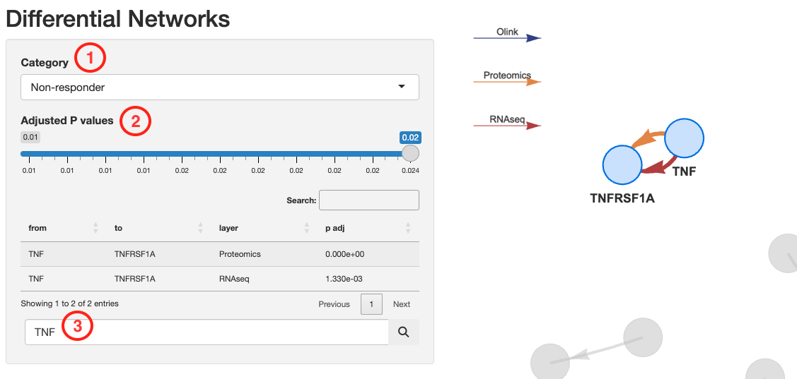
Thicker links correspond to higher significant p-values.
The direction of the arrows shows the relationship direction reported in literature, not derived from the data.

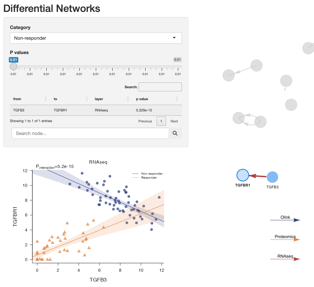
The user can visualize differential regression plots by clicking on a link:

Single node differential expressions can also be visualized by clicking on the nodes:

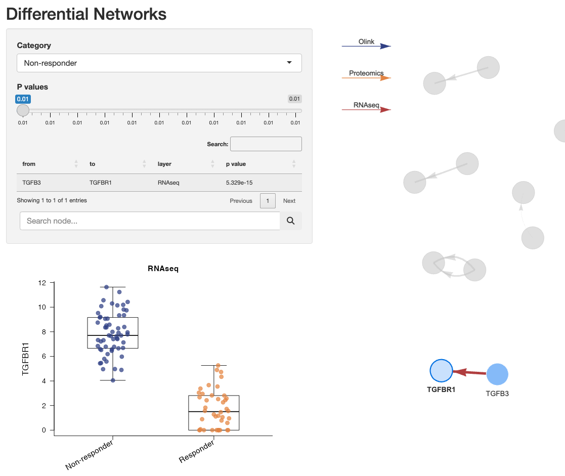
NOTE: For multi-omic scenarios, the data from the first matrix in the list passed to assayData will be used for this boxplot.

List All Differential Interactions

Outside of the interactive environment, the get_multiOmics_diffNetworks() function can be used to get a table of all differential interactions, ordered by p-value or adjusted p-value:

get_multiOmics_diffNetworks(deggs_object, sig_threshold = 0.05)
#> $Non_responder
#>                  from       to      p.value        p.adj      layer
#> TNF-TNFRSF1A      TNF TNFRSF1A 3.325023e-04 1.330009e-03     RNAseq
#> IL1B-IL1R2       IL1B    IL1R2 5.389195e-04 2.155678e-03     RNAseq
#> TGFB3-TGFBR1    TGFB3   TGFBR1 5.329071e-15 2.131628e-14     RNAseq
#> AKT2-MTOR        AKT2     MTOR 4.347083e-04 1.738833e-03     RNAseq
#> FANCD2-FAN1    FANCD2     FAN1 4.440892e-16 3.552714e-15 Proteomics
#> GNG12-RASA2     GNG12    RASA2 0.000000e+00 0.000000e+00 Proteomics
#> RASGRP3-RRAS  RASGRP3     RRAS 2.202344e-04 1.761875e-03 Proteomics
#> TNF-TNFRSF1A1     TNF TNFRSF1A 0.000000e+00 0.000000e+00 Proteomics
#> RASGRP1-RAP1A RASGRP1    RAP1A 2.840564e-03 2.272452e-02 Proteomics
#> 
#> $Responder
#>                from    to      p.value        p.adj  layer
#> FANCD2-FAN1  FANCD2  FAN1 0.000000e+00 0.000000e+00 RNAseq
#> FASLG-FAS     FASLG   FAS 6.947839e-07 2.084352e-06 RNAseq
#> MAP2K2-MAPK3 MAP2K2 MAPK3 1.153300e-12 3.459899e-12 RNAseq

For single omic scenarios, use the get_sig_deggs() function:

deggs_object_oneOmic <- get_diffNetworks(assayData = synthetic_rnaseqData,
                                 metadata = synthetic_metadata,
                                 category_variable = "response",
                                 regression_method = "lm",
                                 padj_method = "bonferroni",
                                 verbose = FALSE,
                                 show_progressBar = FALSE,
                                 cores = 2)

get_sig_deggs(deggs_object_oneOmic, sig_threshold = 0.05)
#>                              from       to      p.value        p.adj
#> Non_responder.TNF-TNFRSF1A    TNF TNFRSF1A 3.325023e-04 1.330009e-03
#> Non_responder.IL1B-IL1R2     IL1B    IL1R2 5.389195e-04 2.155678e-03
#> Non_responder.TGFB3-TGFBR1  TGFB3   TGFBR1 5.329071e-15 2.131628e-14
#> Non_responder.AKT2-MTOR      AKT2     MTOR 4.347083e-04 1.738833e-03
#> Responder.FANCD2-FAN1      FANCD2     FAN1 0.000000e+00 0.000000e+00
#> Responder.FASLG-FAS         FASLG      FAS 6.947839e-07 2.084352e-06
#> Responder.MAP2K2-MAPK3     MAP2K2    MAPK3 1.153300e-12 3.459899e-12

Differential Regression Plots

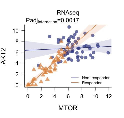
To plot the differential regression fits outside of the interactive environment, use plot_regressions() specifying the omic data to be used and the two targets:

plot_regressions(deggs_object,
                 assayDataName = "RNAseq",
                 gene_A = "MTOR", 
                 gene_B = "AKT2",
                 legend_position = "bottomright")

In single omic analyses, the assayDataName parameter can remain unset.

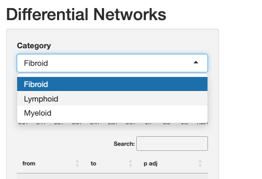
Differential Network Analysis with More Than Two Groups

It’s possible to compare differential interactions among more than two categorical groups. All steps described above stay the same;
the dropdown menu of the interactive environment will show all available categories:

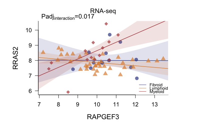
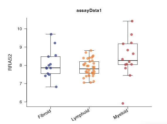
While regressions and boxplots will show all categories:

The statistical significance of the interaction term is calculated via one-way ANOVA in this case.
We highly recommend to have at least 4 or 5 observations per group.

Feature Selection and Engineering with multiDEGGs in Nested Cross-Validation

In computational biology applications involving high-throughput data, researchers commonly encounter situations where the number of potential predictors far exceeds the available sample size. This dimensional challenge requires careful feature selection strategies for both mathematical and clinical reasons.

Standard feature selection methods typically evaluate predictors individually, identifying those variables that show the strongest univariate associations with the outcome variable (such as through t-tests or Wilcoxon tests). While effective, this approach overlooks the interconnected nature of biological systems, where

Feature engineering represents a complementary strategy that creates new predictors by combining or transforming existing variables. In biology, such approach can be used to capture higher-order information that reflects the interconnected nature of molecular processes. For instance, the ratio between two genes may provide more discriminative power than either gene expression level independently, particularly when their relative balance is disrupted in disease states.

The informative content encoded in differential interactions, combined with multiDEGGs’ ability to identify only literature-validated differential relationships, makes it particularly well-suited for both individual feature selection and guided creation of engineered predictors in machine learning. Such approach has potential to overcome the limitations of conventional algorithms which may select individual predictors without clear biological significance, compromising both the interpretability and clinical credibility of the resulting models.

Why Nested Cross-Validation for Feature Engineering?

It is crucial that feature selection and modification is conducted exclusively on training data within cross-validation loops to prevent information leakage from the test set. The nestedcv package enables the nested modification of predictors within each outer fold, ensuring that the attributes learned from the training part are applied to the test data without prior knowledge of the test data itself.
The selected and combined features, and corresponding model, can then be evaluated on the hold-out test data without introducing bias.

Both (nestcv.glmnet) and (nestcv.train) from nestedcv accept any user-defined function that filters or transforms the feature matrix by passing the function name to the modifyX parameter.
The multiDEGGs package provides two specialized functions for this purpose.

multiDEGGs_filter(): Pure Differential Network-Based Selection

The multiDEGGs_filter() function performs feature selection based entirely on differential network analysis. It identifies significant differential molecular interactions and can return either the interaction pairs alone or both pairs and individual variables involved in those interactions.

Key Parameters

When using multiDEGGs_filter(), you can control the following parameters through modifyX_options:

keep_single_genes (logical, default FALSE): Controls whether to include individual genes from significant pairs in addition to the pairs themselves
nfilter (integer, default NULL): Maximum number of predictors to return. When NULL, all significant interactions found are included

Usage Examples

Basic Usage: Pairs Only

library(nestedcv)
data("synthetic_metadata")
data("synthetic_rnaseqData")

# Regularized linear model with interaction pairs only
fit.glmnet <- nestcv.glmnet(
  y = as.numeric(synthetic_metadata$response),
  x = t(synthetic_rnaseqData),
  modifyX = "multiDEGGs_filter",
  modifyX_options = list(
    keep_single_genes = FALSE,
    nfilter = 20
  ),
  modifyX_useY = TRUE,
  n_outer_folds = 5,
  n_inner_folds = 6,
  verbose = FALSE
)

summary(fit.glmnet)
#> Nested cross-validation with glmnet
#> No filter
#> Modifier:  multiDEGGs_filter 
#> Outer loop:  5-fold CV
#> Inner loop:  6-fold CV
#> 100 observations, 14 predictors
#> 
#>        alpha  lambda n.filter
#> Fold 1   0.2 0.16011        7
#> Fold 2   0.1 0.07423        7
#> Fold 3   0.1 0.14076        7
#> Fold 4   0.1 0.13511        7
#> Fold 5   1.0 0.15091        7
#> 
#> Final parameters:
#>  lambda    alpha  
#> 0.07099  0.10000  
#> 
#> Final coefficients:
#>  (Intercept) TNF:TNFRSF1A    AKT2:MTOR   IL1B:IL1R2    FASLG:FAS TGFB3:TGFBR1 
#>     1.808953    -0.188626    -0.113628     0.050012    -0.034766    -0.030783 
#> MAP2K2:MAPK3  FANCD2:FAN1 
#>    -0.020656    -0.008568 
#> 
#> Result:
#>        RMSE     R.squared   Pearson.r^2           MAE   
#>     0.48505       0.03419       0.04929       0.46076

Including Individual Genes (keep_single_genes = TRUE)

# Random forest model including both pairs and individual genes
fit.rf <- nestcv.train(
  y = synthetic_metadata$response,
  x = t(synthetic_rnaseqData),
  method = "rf",
  modifyX = "multiDEGGs_filter",
  modifyX_options = list(
    keep_single_genes = TRUE,
    nfilter = 30
  ),
  modifyX_useY = TRUE,
  n_outer_folds = 5,
  n_inner_folds = 6,
  verbose = FALSE
)
#> Loading required package: ggplot2
#> Loading required package: lattice

fit.rf$summary
#>                Reference
#> Predicted       Non_responder Responder
#>   Non_responder            57         1
#>   Responder                 1        41
#> 
#>               AUC            Accuracy   Balanced accuracy   
#>            0.9988              0.9800              0.9795

# Plot ROC on outer folds
plot(fit.rf$roc)

How nfilter works with keep_single_genes

When keep_single_genes = FALSE: nfilter limits only the number of interaction pairs returned
When keep_single_genes = TRUE: nfilter limits the combined count of unique individual genes plus interaction pairs. The function prioritizes pairs by significance and adds individual genes as needed until the limit is reached

multiDEGGs_combined_filter(): Hybrid Statistical and Network-Based Selection

The multiDEGGs_combined_filter() function combines traditional statistical feature selection with differential network analysis. This hybrid approach allows you to benefit from both conventional univariate selection methods and the biological insights from interaction analysis.

Key Parameters

filter_method (character): Statistical method for single feature selection.
Options: "ttest", "wilcoxon", "ranger", "glmnet", "pls"
nfilter (integer): Maximum number of features to select
dynamic_nfilter (logical): Controls how nfilter is applied (see detailed explanation below)
keep_single_genes (logical): When dynamic_nfilter = TRUE, determines whether to include individual genes from multiDEGGs pairs

Dynamic vs. Balanced Selection Modes

Dynamic Selection (`dynamic_nfilter = TRUE`)

In dynamic mode, the function: 1. Selects nfilter single genes using the chosen statistical method 2. Adds ALL significant interaction pairs found by multiDEGGs 3. Total predictors = nfilter single genes + number of significant pairs

This mode allows the feature space to expand based on the biological complexity discovered in each fold.

# Dynamic selection with t-test for single genes
fit.dynamic <- nestcv.glmnet(
  y = as.numeric(synthetic_metadata$response),
  x = t(synthetic_rnaseqData),
  modifyX = "multiDEGGs_combined_filter",
  modifyX_options = list(
    filter_method = "ttest", 
    nfilter = 20,
    dynamic_nfilter = TRUE, 
    keep_single_genes = FALSE
  ),
  modifyX_useY = TRUE,
  n_outer_folds = 5,
  n_inner_folds = 6,
  verbose = FALSE
)

Balanced Selection (`dynamic_nfilter = FALSE`)

In balanced mode, the function:
1. Allocates approximately half of nfilter to interaction pairs
2. Fills remaining slots with single genes from the statistical filter
3. Maintains consistent total number of predictors across all folds

This mode ensures a fixed feature space size while balancing single genes and interactions.

# Balanced selection with Wilcoxon-test importance
fit.balanced <- nestcv.train(
  y = synthetic_metadata$response,
  x = t(synthetic_rnaseqData),
  method = "rf",
  modifyX = "multiDEGGs_combined_filter",
  modifyX_options = list(
    filter_method = "wilcoxon", 
    nfilter = 40,
    dynamic_nfilter = FALSE
  ),
  modifyX_useY = TRUE,
  n_outer_folds = 5,
  n_inner_folds = 6,
  verbose = FALSE
)

Available Statistical Methods

"ttest": Two-sample t-test for differential expression
"wilcoxon": Wilcoxon rank-sum test (non-parametric alternative to t-test)
"ranger": Random Forest variable importance scoring (the ranger package must be installed first)
"glmnet": Elastic net regularization coefficients
"pls": Partial Least Squares variable importance

Practical considerations

Before implementing multiDEGGs in your machine learning pipeline, it’s highly recommended to first run a preliminary analysis on your complete dataset to assess the number of differential interactions detected. This exploratory step can guide your choice of approach and parameter settings.

If multiDEGGs identifies only a small number of differential interactions (e.g., fewer than 10-20 pairs), these features alone may lack sufficient predictive power. In such cases, consider:

Using multiDEGGs_combined_filter() to integrate network-based features with traditional statistical selection methods
Setting keep_single_genes = TRUE in multiDEGGs_filter() to include individual genes involved in the differential pairs
Adjusting the percentile_vector or significance thresholds in the initial multiDEGGs analysis to potentially capture more interactions

Conversely, if a large number of differential interactions are detected, multiDEGGs_filter() alone may provide sufficient feature diversity for effective model training.

Feature Engineering Details

Both functions create ratio-based features from significant gene pairs (Gene A / Gene B), which capture the relative expression relationships that drive differential network connectivity. The predict methods automatically handle the feature transformation for both training and test data within each cross-validation fold, ensuring no information leakage.

Note: If no significant differential interactions are found in a particular fold, both functions automatically fall back to t-test-based selection to ensure robust performance across all scenarios. This fallback is indicated by a printed “0” during execution.

Citation

citation("multiDEGGs")
#> To cite package 'multiDEGGs' in publications use:
#> 
#>   Sciacca E, et al. (2023). "DEGGs: An R package with shiny app for the
#>   identification of differentially expressed gene-gene interactions in
#>   high-Throughput sequencing data." _Bioinformatics_, *39*, btad192.
#>   doi:10.1093/bioinformatics/btad192
#>   <https://doi.org/10.1093/bioinformatics/btad192>.
#> 
#> A BibTeX entry for LaTeX users is
#> 
#>   @Article{,
#>     title = {DEGGs: An R package with shiny app for the identification of differentially expressed gene-gene interactions in high-Throughput sequencing data},
#>     author = {Elisabetta Sciacca and {et al.}},
#>     journal = {Bioinformatics},
#>     year = {2023},
#>     volume = {39},
#>     pages = {btad192},
#>     doi = {10.1093/bioinformatics/btad192},
#>   }

Elisabetta Sciacca, Myles Lewis

Introduction

Installation

Quick start - Generate Differential Networks

Key Parameters of get_diffNetworks

Visualization

List All Differential Interactions

Differential Regression Plots

Differential Network Analysis with More Than Two Groups

Feature Selection and Engineering with multiDEGGs in Nested Cross-Validation

Why Nested Cross-Validation for Feature Engineering?

multiDEGGs_filter(): Pure Differential Network-Based Selection

Key Parameters

Usage Examples

Basic Usage: Pairs Only

Including Individual Genes (keep_single_genes = TRUE)

How nfilter works with keep_single_genes

multiDEGGs_combined_filter(): Hybrid Statistical and Network-Based Selection

Key Parameters

Dynamic vs. Balanced Selection Modes

Dynamic Selection (dynamic_nfilter = TRUE)

Balanced Selection (dynamic_nfilter = FALSE)

Available Statistical Methods

Practical considerations

Feature Engineering Details

Citation

Key Parameters of `get_diffNetworks`

Dynamic Selection (`dynamic_nfilter = TRUE`)

Balanced Selection (`dynamic_nfilter = FALSE`)